But before we begin, we need a definition of what we are dealing with. Trading bands are lines plotted in and around the price structure to form an "envelope." It is the action of prices near the edges of the envelope that we are particularly interested in. The earliest reference to trading bands I have come across in technical literature is in The Profit Magic of Stock Transaction Timing; author J.M. Hurst's approach involved the drawing of smoothed envelopes around price to aid in cycle identification.
 

Figure 1 shows an example of this technique: Note in particular the use of different envelopes for cycles of differing lengths.
 

The next major development in the idea of trading bands came in the mid to late 1970s, as the concept of shifting a moving average up and down by a certain number of points or a fixed percentage to obtain an envelope around price gained popularity, an approach that is still employed by many. A good example appears in Figure 2, where an envelope has been constructed around the Dow Jones Industrial Average (DJIA). The average used is a 21-day simple moving average. The bands are shifted up and down by 4%.
 

FIGURE 2:

The procedure to create such a chart is straightforward. First, calculate and plot the desired average. Then calculate the upper band by multiplying the average by 1 plus the chosen percent (1 + 0.04 = 1.04). Next, calculate the lower band by multiplying the average by the difference between 1 and the chosen percent (1 - 0.04 = 0.96). Finally, plot the two bands. For the DJIA, the two most popular averages are the 20- and 21-day averages and the most popular percentages are in the 3.5 to 4.0 range.
 

FIGURE 3:

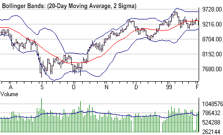
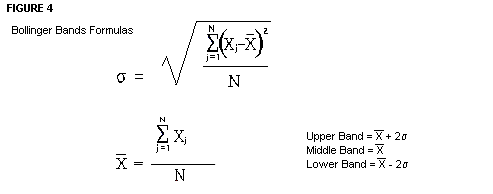
In Figure 5, Bollinger Bands are plotted two standard deviations above and below a 20-day simple moving average. The data used to calculate the standard deviation are the same data as those used for the simple moving average. In essence, you are using moving standard deviations to plot bands around a moving average. The time frame for the calculations is such that it is descriptive of the intermediate-term trend.
 

Note that many reversals occur near the bands and that the average provides support and resistance in many cases.
 

There is great value in considering different measures of price. The typical price, (high + low + close)/3, is one such measure that I have found to be useful. The weighted close, (high + low + close + close)/4, is another. To maintain clarity, I will confine my discussion of trading bands to the use of closing prices for the construction of bands. My primary focus is on the intermediate term, but short- and long-term applications work just as well. Focusing on the intermediate trend gives one recourse to the short- and long-term arenas for reference, an invaluable concept
 

For the stock market and individual stocks. a 20-day period is optimal for calculating Bollinger Bands. It is descriptive of the intermediate-term trend and has achieved wide acceptance. The short-term trend seems well served by the 10-day calculations and the long-term trend by 50-day calculations.
 

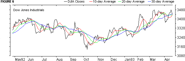
The average that is selected should be descriptive of the chosen time frame. This is almost always a different average length than the one that proves most useful for crossover buys and sells. The easiest way to identify the proper average is to choose one that provides support to the correction of the first move up off a bottom. If the average is penetrated by the correction, then the average is too short. If, in turn, the correction falls short of the average, then the average is too long. An average that is correctly chosen will provide support far more often than it is broken. (See Figure 6.)
 

Bollinger Bands can be applied to virtually any market or security. For all markets and issues, I would use a 20-day calculation period as a starting point and only stray from it when the circumstances compel me to do so. As you lengthen the number of periods involved, you need to increase the number of standard deviations employed. At 50 periods, two and a half standard deviations are a good selection, while at 10 periods one and a half do the job quite well.
 

In most cases, the nature of the periods is immaterial; all seem to respond to correctly specified Bollinger Bands. I have used them on monthly and quarterly data, and I know many traders apply them on an intraday basis.
 

Some older work stated that deviation from a trend as measured by standard deviation from a moving average was used to determine extreme overbought and oversold states. But I recommend the use of trading bands as the generation of buy, sell and continuation signals through the comparison of an additional indicator to the action of price within the bands.
 

If price tags the upper band and indicator action confirms it, no sell signal is generated. On the other hand, if price tags the upper band and indicator action does not confirm (that is, it diverges). we have a sell signal. The first situation is not a sell signal; instead, it is a continuation signal if a buy signal was in effect.
 

It is also possible to generate signals from price action within the bands alone. A top (chart formation) formed outside the bands followed by a second top inside the bands constitutes a sell signal. There is no requirement for the second top's position relative to the first top, only relative to the bands. This often helps in spotting tops where the second push goes to a nominal new high. Of course, the converse is true for lows.
 

Indicator %b lets us compare price action to indicator action. On a big push down, suppose we get to -20 for %b and 35 for relative strength index (RSI). On the next push down to slightly lower price levels (after a rally), %b only falls to 10, while RSI stops at 40. We get a buy signal caused by price action within the bands. (The first low came outside of the bands, while the second low was made inside the bands.) The buy signal is confirmed by RSI, as it did not make a new low, thus giving us a confirmed buy signal.
 

Trading bands and indicators are both good tools, but when they are combined, the resultant approach to the markets becomes powerful. Band width, another indicator derived from Bollinger Bands, may also interest traders. It is the width of the bands expressed as a percent of the moving average. When the bands narrow drastically, a sharp expansion in volatility usually occurs in the very near future. For example, a drop in band width below 2% for the Standard & Poor's 500 has led to spectacular moves. The market most often starts off in the wrong direction after the bands tighten prior to really getting under way, of which January 1991 is a good example (Figure 9).

FIGURE 9:

So one indicator derived from closing prices, another from volume and the last from price range would provide a useful group of indicators. But combining RSI, moving average convergence/divergence (MACD) and rate of change (assuming all were derived from closing prices and used similar time spans) would not. Here are, however, three indicators to use with bands to generate buys and sells without running into problems. Amid indicators derived from price alone, RSI is a good choice. Closing prices and volume combine to produce on-balance volume, another good choice. Finally, price range and volume combine to produce money flow, again a good choice. None is too highly colinear and thus together combine for a good grouping of technical tools. Many others could have been chosen as well: MACD could be substituted for RSI, for example.
 

The Commodity Channel Index (CCI) was an early choice to use with the bands, but as it turned out, it was a poor one, as it tends to be colinear with the bands themselves in certain time frames. The bottom line is to compare price action within the bands to the action of an indicator you know well. For confirmation of signals, you can then compare the action of another indicator, as long as it is not colinear with the first.
 

• Bollinger Bands provide a relative definition of high and low.
   
• That relative definition can be used to compare price action and indicator action to arrive at rigorous buy and sell decisions.
   
• Appropriate indicators can be derived from momentum, volume, sentiment, open interest, inter-market data, etc.
   
• Volatility and trend have already been deployed in the construction of Bollinger Bands, so their use for confirmation of price action is not recommended.
   
• The indicators used for confirmation should not be directly related to one another. Two indicators from the same category do not increase confirmation. Avoid colinearity.
   
• Bollinger Bands can also be used to clarify pure price patterns such as M-type; tops and W-type bottoms, momentum shifts, etc.
   
• Price can, and does, walk up the upper Bollinger Band and down the lower Bollinger Band.
   
• Closes outside the Bollinger Bands can be continuation signals, not reversal signals--as is demonstrated by the use of Bollinger Bands in some very successful volatility-breakout systems.
   
• The default parameters of 20 periods for the moving average and standard deviation calculations, and two standard deviations for the bandwidth are just that, defaults. The actual parameters needed for any given market/task may be different.
   
• The average deployed should not be the best one for crossovers. Rather, it should be descriptive of the intermediate-term trend.
   
• If the average is lengthened the number of standard deviations needs to be increased simultaneously; from 2 at 20 periods, to 2.1 at 50 periods. Likewise, if the average is shortened the number of standard deviations should be reduced; from 2 at 20 periods, to 1.9 at 10 periods.
   
• Bollinger Bands are based upon a simple moving average. This is because a simple moving average is used in the standard deviation calculation and we wish to be logically consistent.
   
• Be careful about making statistical assumptions based on the use of the standard deviation calculation in the construction of the bands. The sample size in most deployments of Bollinger Bands is too small for statistical significance and the distributions involved are rarely normal.
   
• Indicators can be normalized with %b, eliminating fixed thresholds in the process.
   
• Finally, tags of the bands are just that, tags not signals. A tag of the upper Bollinger Band is NOT in-and-of-itself a sell signal. A tag of the lower Bollinger Band is NOT in-and-of-itself a buy signal.
   

  John Bollinger, CFA,CMT

  © John Bollinger 2001