There are many indicators available to measure volume and the flow of money for a particular stock, index or security. One of the most popular volume indicators over the years has been the Accumulation/Distribution Line. The basic premise behind volume indicators, including the Accumulation/Distribution Line, is that volume precedes price. Volume reflects the amount of shares traded in a particular stock and is a direct reflection of the money flowing into and out of a stock. Many times before a stock advances, there will be period of increased volume just prior to the move. Most volume or money flow indicators are designed to identify early increases in positive or negative volume flow to gain an edge before the price moves. (Note: the terms "money flow" and "volume flow" are essentially interchangeable.)

The Accumulation/Distribution Line was developed by Marc Chaikin to assess the cumulative flow of money into and out of a security. In order to fully appreciate the methodology behind the Accumulation/Distribution Line, it may be helpful to examine one of the earliest volume indicators and see how it compares.

In 1963, Joe Granville developed On Balance Volume (OBV), which was one of the earliest and most popular indicators to measure positive and negative volume flow. OBV is a relatively simple indicator that adds the corresponding period's volume when the close is up and subtracts it when the close is down. A cumulative total of the positive and negative volume flow (additions and subtractions) forms the OBV line. This line can then be compared with the price chart of the underlying security to look for divergences or confirmation.

In developing the Accumulation/Distribution Line, Chaikin took a different approach. OBV uses the change in closing price from one period to the next to value the volume as positive or negative. Even if a stock opened on the low and closed on the high, the period's OBV value would be negative as long as the close was lower than the previous period's close. Chaikin chose to ignore the change from one period to the next and instead focused on the price action for a given period (day, week, month). He derived a formula to calculate a value based on the location of the close, relative to the range for the period. We will call this value the "Close Location Value" or CLV. The CLV ranges from plus one to minus one with the center point at zero. There are basically five combinations:

1. If the stock closes on the high, the absolute top of the range, then the value would be plus one.
2. If the stock closes above the midpoint of the high-low range, but below the high, then the value would be between zero and one.
3. If the stock closes exactly halfway between the high and the low, then the value would be zero.
4. If the stock closes below the midpoint of the high-low range, but above the low, then the value would be negative.
5. If the stock closes on the low, the absolute bottom of the range, then the value would be minus one.

The CLV is then multiplied by the corresponding period's volume and the cumulative total forms the Accumulation/Distribution Line.

Ciena

The daily chart of CIEN gives a breakdown of the Accumulation/Distribution Line and shows how different closing levels affect the value. The top section shows the price chart for CIEN. The closing level relative to the high-low range is clearly visible. The second section with a black histogram is the Closing Location Value (CLV). The CLV is multiplied by volume and the result appears in the green histogram. Finally, at the bottom, is the Accumulation/Distribution Line.

1. The close is on the low and the CLV = -1. Volume, however, was relatively light and the Accumulation/Distribution Value for that period is only moderately negative.
2. The close is very near the high and the CLV = +.9273. Volume is relatively high and the resulting Accumulation/Distribution Value is high.
3. The close is near the low and the CLV = -.75. Volume is moderately high and the resulting Accumulation/Distribution Value is moderately high as well.
4. The close is about half way between the mid-point of the high-low range and the high, and the CLV = +.51. Volume is very heavy and the Accumulation/Distribution Value is also very high.

The signals for the Accumulation/Distribution Line are fairly straightforward and center around the concepts of divergence and confirmation.

A bullish signal is given when the Accumulation/Distribution Line forms a positive divergence. Be wary of weak positive divergences that fail to make higher reaction highs or those that are relatively young. The main issue is to identify the general trend of the Accumulation/Distribution Line. A two-week positive divergence may be a bit suspect. However, a multi-month positive divergence deserves serious attention.

Alcoa

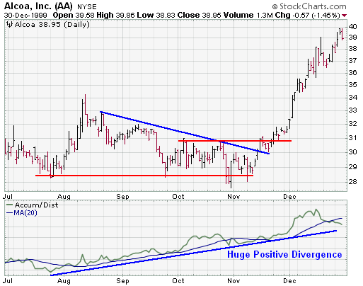
On the chart for AA, the Accumulation/Distribution Line formed a huge positive divergence that was over 4 months in the making. Even though the stock fell from above 35 to below 30, the Accumulation/Distribution Line continued on a relentless march north. If one did not know better, it would seem that the two plots did not belong together. However, the stock finally caught up with the Accumulation/Distribution Line when it broke resistance in November.

Another means of using the Accumulation/Distribution Line is to confirm the strength or sustainability behind an advance. In a healthy advance, the Accumulation/Distribution Line should keep up or at the very least move in an uptrend. If the stock is moving up at a rapid clip, but the Accumulation/Distribution Line has trouble making higher highs or trades sideways, it should serve as an indication that buying pressure is relatively weak.

Walmart

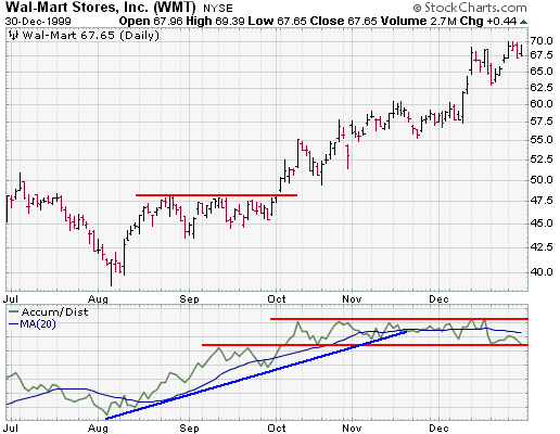
WMT began a sharp advance in August that was accompanied by an equally strong move in the Accumulation/Distribution Line. In fact, the Accumulation/Distribution Line was stronger than the stock in early September. After a bit of a consolidation, both again started higher and recorded new reaction highs in early October. Volume flows were behind this advance from the very beginning and continued throughout. The stock ended up advancing from 40 to 60 in about 3 months. Interestingly, as of this writing (December 1999) the Accumulation/Distribution Line has started to move sideways and is indicating that buying pressure is beginning to wane.

The same principles that apply to positive divergences apply to negative divergences. The key issue is to identify the main trend in the Accumulation/Distribution Line and compare it to the underlying security. Young negative divergences, or those that are relatively flat, should be looked upon with a healthy dose of skepticism.

The WMT chart shows a relatively flat negative divergence that is just over a month old. This negative divergence has yet to make a lower low and should probably be given a little more time to mature. The relative weakness in the Accumulation/Distribution Line should serve as a sign that buying pressure is diminishing while the stock remains at lofty levels.

Delta Airlines

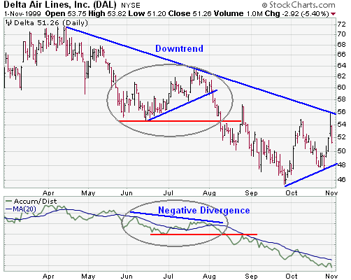
The DAL chart shows a negative divergence that developed within the confines of a clear downtrend. The stock had clearly broken down and the Accumulation/Distribution Line was declining in line with the stock. A deteriorating Accumulation/Distribution Line confirmed weakness in the stock. During the June-July rally, the stock recorded a new reaction high, but the Accumulation/Distribution Line failed, thus setting up the negative divergence.